
Searching Isn’t the Hard Part — Matching Is
The first version of search in almost any product looks the same. Somebody sits down one afternoon, writes this, and calls it done:
SELECT *FROM postsWHERE content ILIKE '%postgres%';And for a while, it’s fine. The table’s small, the queries are honest, nobody’s filing a bug about it.
Then the product grows up, and so do the requests. Users search for running when the post says run. They type database indexing because both words are in the doc, even though they’re not next to each other. They search in title case, all caps, and once, with a typo they don’t notice. Every one of those is a reasonable person doing their best, and every one of them gets told “nothing matches.”
That’s the moment ILIKE '%query%' stops looking like search and starts looking like “read the whole table and hope.”
The part that’s easy to miss is that this was never about that one query being slow. Throw five million rows at it and ILIKE doesn’t get any smarter. There’s no structure anywhere that says:
database → rows 4, 18, 73, 91, 1042, ...The database just walks every row and asks the same question, one at a time:
Row 1 → does body contain "database"?Row 2 → does body contain "database"?Row 3 → does body contain "database"?Row 4 → does body contain "database"?...A plain B-tree index doesn’t rescue you either. B-trees are excellent for WHERE id = 123 or WHERE email = 'foo@example.com' — exact, left-anchored lookups. A wildcard in the middle of the string is precisely the one shape a B-tree can’t answer.
Note
The deeper problem isn’t speed — it’s language. running and run are different strings but the same concept, and substring matching can’t see that. “The system is running efficiently” should match a search for run; a literal scan will never agree.
So we don’t really want to search raw text at all. We want a normalized representation of it, and then we search that. Everything else in this post is an argument for that one move.
Part 1: Turning Documents Into Something Searchable
Instead of storing this:
"The quick brown fox jumps over the lazy dog."we preprocess it into something closer to:
quickbrownfoxjumplazidogNow flip the mapping — word → documents instead of document → words:
quick → 1, 7, 42 brown → 1, 19, 42 fox → 1, 5, 42 jump → 1, 8, 42 database → 3, 9, 17, 100 postgres → 4, 10, 27That’s the inverted index, and it’s the core idea behind essentially every modern lexical search engine, Elasticsearch included. It analyzes text, builds term → documents, executes against that structure, and ranks what comes back.
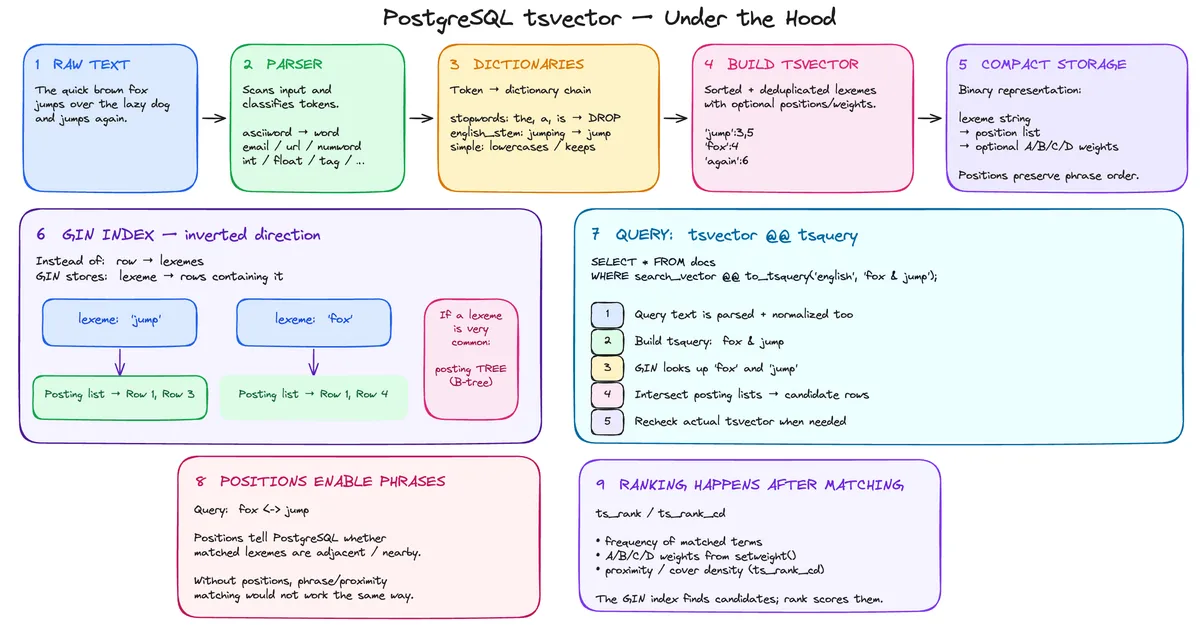
Postgres can do all of that too — it just calls the pieces different things. The central one is tsvector.
Part 2: tsvector, and Where Those Lexemes Come From
Postgres defines tsvector as a representation of a document optimized for text search — in practice, a sorted list of distinct, normalized lexemes, each with optional position and weight info. The phrasing is worth reading twice, because it does not say “a special column full of words.”
Concrete example, because that definition is dry:
SELECT to_tsvector( 'english', 'The quick brown fox jumps and jumps again');Conceptually you get:
'again':8'brown':3'fox':4'jump':5,7'quick':2The sentence has become a lexeme → positions map. 'jump':5,7 means the word showed up twice, at positions 5 and 7, and is stored as one entry instead of two. If you keep one picture from this post, this is it:
Document   ↓Normalized searchable representation
{    again → [8]    brown → [3]    fox   → [4]    jump  → [5,7]    quick → [2]}
Where the Lexemes Come From
to_tsvector() isn’t split(" ") with extra steps. The pipeline has real stages:
TEXT │ ▼ ┌─────────┐ │ Parser │ → what kind of thing is this? └────┬────┘ │ token + type ▼ ┌─────────────────┐ │ Configuration │ → token type → dictionary mapping └────────┬────────┘ ▼ Dictionaries → what should it be indexed as? │ ▼ Lexeme(s) │ ▼ tsvectorSplit those two questions apart and a lot of Postgres search stops being magic:
PARSER "What is this piece of text?" ↓DICTIONARY "What should I index it as?"Parser — breaks input into tokens and classifies them. The default parser knows 23 token types, and they’re an odd mix: asciiword, email, url, int, float, version, tag. Feed it foo@bar.com costs $19.99 and it quietly tags the pieces as email, asciiword, and float. ts_debug() shows you the whole thing.
Configuration — decides which dictionaries run for each token type. There’s no reason to treat postgres, someone@example.com, and 192.168.1.1 the same way, so you don’t have to. A dictionary then has a short menu of behaviors: recognize a token and emit lexemes, treat it as a stopword and emit nothing, or pass it on to the next dictionary in the chain.
This is why the pipeline isn’t just tokenization. The full transformation is:
Raw text ↓Tokenization + classification ↓Dictionary chain: ├── stopword? → discard ├── synonym? → replace ├── stemmable? → normalize └── unknown? → next dictionary ↓Lexeme + position + optional weight ↓Sorted + deduplicated ↓tsvectorStopwords and Stemming
Some words — the, a, an, is, of, in — carry almost no signal, so they’re dropped. The subtle part: Postgres doesn’t pretend they were never there. Their positions still leave gaps, and those gaps can matter for proximity-based ranking. For “in the list of stop words” you get:
'list':3 'stop':5 'word':6Positions 1, 2, and 4 are missing — they were stopwords. The words disappear from the lexeme set, but their positional footprint doesn’t necessarily.
Stemming is where running can match run. The built-in English stemmer is a Snowball dictionary:
SELECT ts_lexize('english_stem', 'stars'); -- {star}So both sides of a search can be normalized into the same lexeme, and the comparison happens at the lexeme level, not the string level:
running → runrun → runThat’s one of the fundamental differences between full-text search and substring search — both sides of the comparison get normalized to the same lexeme before the comparison ever happens.
Part 3: Positions and Weights Do More Than They Seem To
Why keep fox → 4 around instead of just fox? Because the position tells the engine where the word was, and that unlocks phrase matching and smarter ranking.
Compare “The fox jumps quickly” with “The fox is somewhere across the field and eventually jumps.” Both contain fox and jump, but in the first they’re adjacent. That’s the difference between:
'fox' & 'jump' both match any two documents'fox' <-> 'jump' lexemes that appear successivelytsquery_phrase() gives you the same control with explicit distances. Positions aren’t shipped around out of politeness — they’re a big part of why Postgres can beat ILIKE '%fox%' here at all.
PostgreSQL also lets you attach weights — A, B, C, D — to positions so a match in a title (weight A) can outrank one buried in the body (weight D):
title: postgres → [1:A]body: postgres → [14:D, 38:D, 92:D]Internally, a tsvector is a sorted, deduplicated set of lexeme → positions entries, with positions capped at 16383. It isn’t a list stored awkwardly as a column; it’s a purpose-built data type, and treating it like one saves you from a whole class of later surprises.
Part 4: GIN Turns the Representation Upside Down
One thing to get straight before we get to the fast part: a tsvector alone doesn’t make search fast. You can search like this:
SELECT *FROM documentsWHERE to_tsvector('english', body) @@ to_tsquery('english', 'database');But on a large table, regenerating tsvector values while scanning every row isn’t the architecture you want. That’s where GIN — the Generalized Inverted Index — comes in.
Suppose your table looks like:
Row 1 → {postgres, database, index}Row 2 → {database, sql}Row 3 → {postgres, search}Row 4 → {database, index}The row-oriented representation is row → terms. GIN builds the inverted one — term → rows:
postgres → [Row 1, Row 3]database → [Row 1, Row 2, Row 4]index → [Row 1, Row 4]sql → [Row 2]search → [Row 3]This is why it’s so much faster. With 10 million documents and only 20,000 containing postgres:
Sequential scan: Inverted index:10,000,000 rows postgres ↓ ↓Does this contain postgres? GIN ↓ ↓(read EVERYTHING) 20,000 candidate rowsThe database has eliminated the other ~9.98 million rows without ever touching them. Under the hood, GIN keeps (key, posting list) pairs — a lexeme pointing at the rows that mention it.
A typical production setup stores the vector so it isn’t recomputed on every query:
ALTER TABLE documentsADD COLUMN search_vector tsvectorGENERATED ALWAYS AS ( to_tsvector( 'english', coalesce(title, '') || ' ' || coalesce(body, '') )) STORED;
CREATE INDEX documents_search_idxON documentsUSING GIN (search_vector);Now your inserts and updates automatically maintain the search representation and the index over it.
Note
One subtlety: GIN stores the lexemes, not the weight labels. When you query on weights, PostgreSQL may need to recheck information that isn’t represented directly in the GIN keys.
Part 5: The Other Half — tsquery and @@
We have the document representation (tsvector). Now we need the query representation: tsquery — and it’s worth its own section, because it’s where people get the “why did this query match that document” surprises.
Document → tsvectorQuery → tsqueryA document like “The quick brown fox jumps” becomes 'quick':2 'brown':3 'fox':4 'jump':5. A query like "fox jump" becomes a structured expression over lexemes:
postgres & database    →      AND                             /    \                       postgres  database
postgres | mysql       →      OR                             /   \                       postgres mysql
!postgres              →     NOT                              │                          postgres
'fox' <-> 'jump'       →     fox immediately followed by jump
The query grammar gives you &, |, !, and <-> — boolean and phrase matching. The engine isn’t testing string contains string; it’s evaluating a structured expression against a normalized index.
And here’s the requirement everyone eventually trips on: the query has to go through the same pipeline as the document. If the document’s running became run at index time, the user’s running also has to become run at query time — otherwise you’re comparing run == running and wondering why nothing matches.
During @@, PostgreSQL intersects posting lists:
fox & jump / \ / \ fox postings jump postings {1,5,8,12,20} {1,3,8,15} \ / INTERSECT {1, 8}Only rows 1 and 8 contain both. Phrase queries (fox <-> jump) then use positions to distinguish “rows with both words” from “rows where the words are actually adjacent” — which is precisely why positions exist.
Part 6: Matching and Relevance Are Two Different Jobs
GIN answers the question “which rows contain these lexemes?” It explicitly does not answer “which matches deserve to be on top?” — that’s a whole separate layer, and conflating the two is a common source of “why is this result first?” confusion.
Postgres pairs the two of them with ts_rank() and ts_rank_cd() to score candidates after matching:
GIN → "Which documents match?" ↓ts_rank / cd → "Of the matches, which matter more?"Roughly, ranking weighs term frequency (a term appearing several times scores higher), position weights (A–D), and — for ts_rank_cd — cover density, which rewards matches that sit close together.
Part 7: PostgreSQL vs Elasticsearch — the Actual Decision
By now, Postgres looks uncomfortably similar to Elasticsearch. It should — at the information-retrieval level they’re solving the same problem with the same shape.
Elasticsearch:                    PostgreSQL:
text analysis                     parser   ↓                                ↓tokens                            dictionaries   ↓                                ↓inverted index                    tsvector   ↓                                ↓query                             GIN   ↓                                ↓relevance scoring                 tsquery                                      ↓                                  ts_rank
Both of them do full-text search well. So the interesting question isn’t “which one understands search” — it’s “how much search infrastructure does your application actually need?” And I’d argue most products need dramatically less than the industry assumes.
For a small-to-medium application, your data (users, posts, products, documents, comments, a knowledge base — whatever the product is about) almost certainly already lives in Postgres. Adding Elasticsearch means standing up an entire second system and with it an entirely new job description nobody asked for:
                Application                    │             ┌──────┴──────┐             ▼             ▼        PostgreSQL     Elasticsearch             │             │          primary        search           data          index
How does data get from PostgreSQL → Elasticsearch?What if indexing fails?   How do we retry?How do we handle stale documents?How do we synchronize deletes?How do we monitor, deploy, back up, and scale a cluster?
With Postgres full-text search, the data and the search index live in the same database system:
Application │ ▼ PostgreSQL / \ data GIN indexOperationally, that’s a dramatically simpler story — and you still get stemming, stopwords, phrase and boolean queries, positional matching, weighted fields, relevance ranking, and indexed search, all without running a search cluster.
Note
The rule I’d actually defend: if you already run Postgres and need conventional lexical search, start with tsvector + GIN. You don’t need Elasticsearch because your app has search. You need it only when the search problem itself gets complex enough to justify a dedicated system — and until then, a second datastore is a tax, not a feature.
But Postgres Isn’t “Elasticsearch in Disguise”
I want to be honest about the ceiling too, because this is where people overshoot in the other direction. Elasticsearch is a dedicated search engine built on Lucene, with fuzzy matching, prefix queries, autocomplete, multi-field search, intervals, and BM25 relevance by default.
Postgres’s ranking functions are different. ts_rank is not BM25 and doesn’t pretend to be — both are relevance approximations, but they aren’t numerically equivalent, and that gap starts to matter the moment relevance is a core product feature rather than a nice-to-have.
Here’s the comparison I’d actually carry around:
| Requirement | PostgreSQL tsvector + GIN | Elasticsearch |
|---|---|---|
| Basic full-text search | Excellent | Excellent |
| Stemming / stopwords | Yes | Yes |
| Phrase / boolean search | Yes | Yes |
| Field weighting | Yes | Yes |
| Relevance ranking | Yes | More sophisticated |
| BM25 | No | Yes (default) |
| Fuzzy search | Limited | Strong |
| Autocomplete | Possible, not its strength | Strong |
| Operational complexity | Low (if already on PG) | Higher |
| Separate infrastructure | No | Yes |
| Distributed search | Not its purpose | Core strength |
| Best for | DB-centric app search | Search-heavy systems |
Part 8: The Whole System in One Trace
Let’s run one query end to end. Document: “PostgreSQL makes database searching fast. PostgreSQL provides powerful indexing.”
1. Raw text → PostgreSQL makes database searching fast. ...2. Parser → each word classified as asciiword3. Dictionaries → postgresql, make, database, search, fast, postgresql, provid, power, index4. tsvector → 'database':3 'fast':5 'index':9 'make':2 'postgresql':1,6 'power':8 'provid':7 'search':45. GIN → postgresql → [Row 17, 42, 91, ...] database → [Row 17, 25, ...]6. User searches → "postgresql database" ⇒ postgresql & database7. GIN lookup → intersect posting lists ⇒ candidate rows8. Ranking → ts_rank / ts_rank_cd ⇒ ordered resultsThe cleanest mental model separates three distinct jobs:
┌──────────────────────────────┐│ DOCUMENT UNDERSTANDING ││ TEXT → Parser + Dicts ││ → tsvector │└──────────────┬───────────────┘ │ ▼┌──────────────────────────────┐│ SEARCH ACCELERATION ││ GIN ││ → candidate rows │└──────────────┬───────────────┘ │ ▼┌──────────────────────────────┐│ RELEVANCE ││ ts_rank / ts_rank_cd ││ → ranked results │└──────────────────────────────┘And there it is. tsvector is not the index — it’s the normalized representation of a document. GIN is the inverted index built over that representation. tsquery is a structured version of the user’s search, @@ does the matching, and ts_rank/ts_rank_cd decide what surfaces first.
DOCUMENT SIDE QUERY SIDERaw text │ User query ↓ │ ↓Parser │ tsquery ↓ │ ↓Dictionaries │ GIN lookup ↓ │ ↓tsvector │ ─────────────── ↓ │ Matching rowsGIN │ ↓ │ ts_rank / cd │ ↓ │ Ranked resultsPostgres already contains all the raw material of a lexical search engine — text analysis, normalized lexemes, positional information, an inverted index, query expressions, and relevance scoring — so it can deliver genuinely capable search without standing up a search cluster.
For a small-to-medium application whose data already lives in Postgres, that’s a pragmatic, defensible choice. The moment search becomes a specialized subsystem — fuzzy matching with real tuning, aggressive autocomplete, relevance you’re shipping as a feature, or a workload that wants to sit across many machines — a dedicated engine earns its keep. Getting that line right is most of the battle, and for a surprising number of products, it lands well to the Postgres side of it.