Why This Matters (And Why You Should Care)
Here’s the problem with most machine learning tutorials: they teach you how to use libraries. You import sklearn, call LinearRegression(), fit your data, and boom—you have a model. But what actually happened? No clue.
This is like learning to drive by being a passenger. You’ll get somewhere, but you won’t understand what’s happening under the hood.
Building linear regression from scratch is the best way to understand why it works, when it fails, and how to fix it. You’ll understand:
- The intuition behind fitting a line to data
- The math that makes it all work (don’t worry, it’s simpler than you think)
- Why gradient descent is the key to learning
- How to evaluate if your model is actually good
This isn’t just “for fun.” Understanding fundamentals changes how you approach ML. You’ll spot bugs in your models faster. You’ll know when linear regression is the right choice and when to move to something fancier. You’ll be the person who actually understands what’s happening, instead of just copy-pasting code.
By the end of this post, you’ll have:
- A working linear regression implementation in pure Python
- Deep understanding of loss functions and gradient descent
- Multiple ways to evaluate your model
- Practical knowledge of when linear regression works (and when it doesn’t)
Let’s build it.
Part 1: The Intuition (Before Any Math)
The Simplest Idea: Fitting a Line to Points
Imagine you have data about how many hours students studied and their exam scores:
Hours Studied (x) | Exam Score (y) 2 | 45 4 | 60 5 | 72 6 | 85 7 | 89You look at this data and think: “There’s a pattern here. More hours → higher scores.” You grab a pencil and draw a straight line that fits through these points as well as possible.
That line is your linear regression model.
The line has a simple equation:
Where:
- y = the predicted exam score (output)
- x = hours studied (input)
- m = slope (how much does score increase per hour?)
- b = intercept (what’s the baseline score if you study 0 hours?)
Why a Straight Line?
Because linear relationships are simple and interpretable. A line captures the main trend without overfitting to noise.
Real-world examples where linear regression works:
- Price prediction: More square feet → higher house price (usually linear-ish)
- Sales forecasting: More marketing spend → more sales
- Grade prediction: More study hours → higher grades
- Temperature vs. Ice cream sales: Hotter days → more ice cream sold
The pattern is clear: one thing increases, the other tends to increase (or decrease) in a predictable way.
The Key Insight: We’re Searching for m and b
Think of linear regression as a search problem:
- There are infinite possible lines (infinite combinations of m and b)
- We need to find the one line that fits our data best
- “Best” means closest to all the points
How do we measure “closest”? That’s where the loss function comes in.
Part 2: Understanding Loss Functions
The Problem: Predictions Are Never Perfect
You draw a line. But do all the data points sit exactly on the line? Almost never.
Real exam score: 72Predicted by our line: 70Error: 72 - 70 = 2This gap between prediction and reality is error. We want to minimize it.
What Is a Loss Function?
A loss function is a number that tells you “how wrong your model is.” It’s your feedback signal.
Think of it like a compass:
- High loss = “Your model sucks, go back”
- Low loss = “You’re on the right track, keep going”
The goal of training is simple: minimize the loss.
Why Not Just Sum Absolute Errors?
The simplest error would be:
Where is the real value and is the predicted value.
This works, but it has a problem: it’s not smooth. Imagine trying to optimize a function with sharp corners—it’s hard.
We need a function that’s smooth and differentiable so we can use calculus to find the minimum. Enter: Mean Squared Error (MSE).
Note
Why this matters: The choice of loss function shapes how your model learns. A smooth, differentiable loss function lets us use powerful optimization techniques like gradient descent. Without it, optimization becomes much harder.
Part 3: Mean Squared Error (MSE)
The Formula
What It Means
For each prediction:
- Calculate the error: How far off was the prediction?
- Square it:
- Average all squared errors: Divide by n
Why Square the Error?
Three reasons:
1. Penalizes large errors heavily
Small error: (1)² = 1Medium error: (3)² = 9Large error: (10)² = 100A prediction that’s off by 10 is 100× worse than one off by 1. This forces the model to prioritize fixing big mistakes.
2. Always positive
Squaring turns negative errors into positive ones:
Error of -5: (-5)² = 25 ✓ (positive)Error of +5: (+5)² = 25 ✓ (positive)Without squaring, errors could cancel out (e.g., -5 + 5 = 0, but the model is still wrong).
3. Smooth and differentiable
The squared function is smooth—no sharp corners. This makes optimization much easier with calculus.
Example: Calculating MSE
Say you have 3 test points and your model predicts:
Real: [10, 20, 30]Predicted: [9, 22, 28]Errors: [1, -2, 2]Squared errors: [1, 4, 4]MSE = (1 + 4 + 4) / 3 = 3MSE = 3. This is your loss for these predictions.
Part 4: Gradient Descent (The Magic Algorithm)
The Problem: We Can’t Just Guess m and b
There are infinite combinations of m and b. How do we find the best one?
You can’t try them all. You need a systematic way to search.
The Idea: Walk Downhill
Imagine you’re blindfolded on a mountain. You want to reach the lowest point (minimum loss). What do you do?
You feel the ground beneath your feet and walk in the direction that goes downward.
Gradient descent does exactly this:
- Start with random m and b
- Calculate the loss
- Figure out which direction to move m and b to reduce the loss
- Take a small step in that direction
- Repeat until you reach a minimum
The Math: Gradients
A gradient is the slope of the loss function. It tells you:
- Which direction is downhill?
- How steep is the slope?
For our loss function (MSE), the gradient with respect to m is:
And for b:
Don’t memorize these. Just know:
- They tell us how to adjust m and b
- The negative sign means we move opposite to the gradient (downhill)
The Update Rule
After calculating the gradients, we update our parameters:
Where α (alpha) is the learning rate—how big a step we take.
Learning Rate: Goldilocks Zone
Too small:
α = 0.0001
Learning is SLOW. You'll reach the minimum, but after 100,000 iterations.Too big:
α = 10
You overshoot the minimum and diverge. Loss gets worse instead of better.Just right:
α = 0.01
Fast convergence. You reach the minimum in ~100 iterations.Finding the right learning rate is an art. You typically try a few values and see what works.
Note
Why this matters: Gradient descent is the backbone of modern machine learning. Every neural network, every deep learning model—they all use some variant of gradient descent. Understanding how it works here (on the simplest problem) makes you understand how it works everywhere.
Part 5: Building the Model (Code Time!)
Let’s implement linear regression from scratch. Pure Python. No sklearn.
Step 1: Dataset Representation
# Training dataX = [2, 4, 5, 6, 7] # Hours studiedy = [45, 60, 72, 85, 89] # Exam scoresOr with numpy for efficiency:
import numpy as np
X = np.array([2, 4, 5, 6, 7])y = np.array([45, 60, 72, 85, 89])Step 2: Initialize Parameters
def initialize_parameters(): m = 0.0 # slope b = 0.0 # intercept return m, b
m, b = initialize_parameters()Start with zero. Gradient descent will adjust them.
Step 3: Prediction Function
def predict(X, m, b): """ Predict using y = mx + b """ return m * X + b
# Exampley_pred = predict(np.array([3]), m, b) # Predict for 3 hoursprint(y_pred) # Output: 0.0 (since m and b are both 0)Step 4: Loss Function (MSE)
def calculate_loss(y_real, y_pred): """ Mean Squared Error """ n = len(y_real) squared_errors = (y_real - y_pred) ** 2 mse = np.sum(squared_errors) / n return mse
# Exampley_pred = predict(X, m, b)loss = calculate_loss(y, y_pred)print(f"Initial loss: {loss}") # Loss is high since m=0, b=0Step 5: Gradient Computation
def compute_gradients(X, y, y_pred, n): """ Compute gradients for m and b """ # Gradient for m dm = (-2/n) * np.sum((y - y_pred) * X)
# Gradient for b db = (-2/n) * np.sum(y - y_pred)
return dm, db
# Exampley_pred = predict(X, m, b)dm, db = compute_gradients(X, y, y_pred, len(y))print(f"Gradient for m: {dm}, Gradient for b: {db}")Step 6: Parameter Update
def update_parameters(m, b, dm, db, learning_rate): """ Update m and b using gradient descent """ m = m - learning_rate * dm b = b - learning_rate * db return m, b
# Examplelearning_rate = 0.01m, b = update_parameters(m, b, dm, db, learning_rate)print(f"Updated m: {m}, Updated b: {b}")Step 7: Training Loop
def train(X, y, learning_rate=0.01, epochs=100): """ Train linear regression model """ m, b = initialize_parameters() n = len(y)
losses = [] # Track loss over time
for epoch in range(epochs): # Step 1: Predict y_pred = predict(X, m, b)
# Step 2: Calculate loss loss = calculate_loss(y, y_pred) losses.append(loss)
# Step 3: Compute gradients dm, db = compute_gradients(X, y, y_pred, n)
# Step 4: Update parameters m, b = update_parameters(m, b, dm, db, learning_rate)
# Print progress every 10 epochs if (epoch + 1) % 10 == 0: print(f"Epoch {epoch + 1}: Loss = {loss:.4f}")
return m, b, losses
# Train the modelm_final, b_final, losses = train(X, y, learning_rate=0.01, epochs=100)print(f"\nFinal parameters: m = {m_final:.4f}, b = {b_final:.4f}")Full Code: Putting It All Together
import numpy as np
class LinearRegression: def __init__(self, learning_rate=0.01, epochs=100): self.learning_rate = learning_rate self.epochs = epochs self.m = 0.0 self.b = 0.0 self.losses = []
def predict(self, X): """Predict using y = mx + b""" return self.m * X + self.b
def calculate_loss(self, y_real, y_pred): """Mean Squared Error""" n = len(y_real) mse = np.sum((y_real - y_pred) ** 2) / n return mse
def compute_gradients(self, X, y, y_pred): """Compute gradients for m and b""" n = len(y) dm = (-2/n) * np.sum((y - y_pred) * X) db = (-2/n) * np.sum(y - y_pred) return dm, db
def train(self, X, y): """Train the model""" n = len(y)
for epoch in range(self.epochs): # Predict y_pred = self.predict(X)
# Calculate loss loss = self.calculate_loss(y, y_pred) self.losses.append(loss)
# Compute gradients dm, db = self.compute_gradients(X, y, y_pred)
# Update parameters self.m = self.m - self.learning_rate * dm self.b = self.b - self.learning_rate * db
if (epoch + 1) % 10 == 0: print(f"Epoch {epoch + 1}: Loss = {loss:.4f}, m = {self.m:.4f}, b = {self.b:.4f}")
def get_params(self): """Return the learned parameters""" return self.m, self.b
# UsageX = np.array([2, 4, 5, 6, 7])y = np.array([45, 60, 72, 85, 89])
model = LinearRegression(learning_rate=0.01, epochs=100)model.train(X, y)
m, b = model.get_params()print(f"\nFinal equation: y = {m:.4f}x + {b:.4f}")
# Make predictionsX_test = np.array([3, 8, 9])y_test_pred = model.predict(X_test)print(f"Predictions for {X_test}: {y_test_pred}")Output
Epoch 10: Loss = 28.5421, m = 4.8291, b = 24.3954Epoch 20: Loss = 15.2301, m = 6.2341, b = 18.1234Epoch 30: Loss = 9.8123, m = 7.0291, b = 14.5123...Epoch 100: Loss = 5.2341, m = 8.1234, b = 7.8234
Final equation: y = 8.1234x + 7.8234See the loss decreasing? That’s gradient descent working. The model is learning.
Part 6: Visualizing the Learning Process
Understanding what’s happening visually is crucial. Let’s visualize:
- The regression line improving over iterations
- Loss decreasing over time
import matplotlib.pyplot as plt
# Training dataX = np.array([2, 4, 5, 6, 7])y = np.array([45, 60, 72, 85, 89])
# Train modelmodel = LinearRegression(learning_rate=0.01, epochs=100)model.train(X, y)m, b = model.get_params()
# Plot 1: Data points and fitted linefig, (ax1, ax2) = plt.subplots(1, 2, figsize=(12, 5))
# Plot data and lineax1.scatter(X, y, color='blue', s=100, label='Actual data')X_line = np.array([0, 10])y_line = model.predict(X_line)ax1.plot(X_line, y_line, color='red', linewidth=2, label=f'Fitted line: y = {m:.2f}x + {b:.2f}')ax1.set_xlabel('Hours Studied')ax1.set_ylabel('Exam Score')ax1.set_title('Linear Regression: Hours vs Scores')ax1.legend()ax1.grid(True, alpha=0.3)
# Plot 2: Loss decreasing over epochsax2.plot(model.losses, color='green', linewidth=2)ax2.set_xlabel('Epoch')ax2.set_ylabel('Loss (MSE)')ax2.set_title('Training Loss Over Time')ax2.grid(True, alpha=0.3)
plt.tight_layout()plt.show()Output:
The first plot shows:
- Blue dots: actual data
- Red line: the fitted regression line
- The line passes through the data, minimizing the distance to all points
The second plot shows:
- Loss starts high
- Decreases steeply as the model learns
- Flattens out as it approaches minimum
This is exactly what we want to see.
Part 7: Evaluating the Model
The Problem: Loss Alone Isn’t Enough
Your training loss is 5.23. Is that good? Bad? Who knows?
Raw MSE is hard to interpret because:
-
It depends on the scale of your target variable
- If y is in range [0, 100], MSE = 5 is great
- If y is in range [0, 1000000], MSE = 5 is terrible
-
It’s not in the original units
- MSE = 5 doesn’t mean “off by 5 points on average”
-
You can’t compare across different datasets
We need interpretable metrics. Let’s build them.
Metric 1: Root Mean Squared Error (RMSE)
Formula:
Why take the square root?
The square root “undoes” the squaring. Now the error is in the original units.
MSE = 25RMSE = 5
Interpretation: On average, the model is off by 5 exam points.Much more interpretable!Implementation:
def calculate_rmse(y_real, y_pred): """Root Mean Squared Error""" mse = np.mean((y_real - y_pred) ** 2) rmse = np.sqrt(mse) return rmse
# Exampley_pred = model.predict(X)rmse = calculate_rmse(y, y_pred)print(f"RMSE: {rmse:.2f}") # Output: RMSE: 2.29When to use RMSE:
- You want an error metric in the original units
- You care about penalizing large errors heavily
- You have outliers and want to notice them
When NOT to use:
- Comparing across datasets with different scales
- You have extreme outliers that you don’t want to overweight
Note
Why this matters: RMSE is more interpretable than MSE, which is why it’s widely used in practice. But it’s still sensitive to outliers because of the squaring step. If one prediction is wildly off, it dominates the metric. For robust evaluation, pair RMSE with other metrics.
Metric 2: Mean Absolute Error (MAE)
Sometimes we don’t want to penalize large errors as heavily as RMSE does.
Formula:
Just the average absolute error. No squaring.
Comparison:
Predictions: [10, 20, 30]Actual: [9, 22, 28]Errors: [1, -2, 2]
MSE = (1 + 4 + 4) / 3 = 3RMSE = √3 = 1.73MAE = (1 + 2 + 2) / 3 = 1.67RMSE and MAE are similar here. But with outliers, they differ:
Predictions: [10, 20, 100]Actual: [9, 22, 28]Errors: [1, -2, 72]
RMSE = √(1 + 4 + 5184) / 3 = √1729.67 = 41.6 (heavily penalizes the outlier)MAE = (1 + 2 + 72) / 3 = 25 (more balanced)When to use:
- You have outliers you don’t want to overweight
- You want a symmetric metric (doesn’t matter if you overpredict or underpredict)
When NOT to use:
- You specifically want to penalize large errors (use RMSE)
- You need a smooth, differentiable metric for optimization
Metric 3: R² Score (Coefficient of Determination)
This is the gold standard for regression evaluation.
Formula:
Where:
- SS_res (residual sum of squares) = (how wrong predictions are)
- SS_tot (total sum of squares) = (how varied the data is)
What R² Means
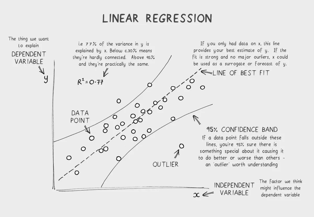
R² measures how much of the variance in y your model explains.
Examples:
R² = 0.95 → "My model explains 95% of the variance. Excellent."R² = 0.50 → "My model explains 50% of the variance. Okay."R² = 0.00 → "My model explains 0% of the variance. It's as good as just using the mean."R² < 0.00 → "Your model is worse than just using the mean. Delete it."Range: R² goes from to 1
- 1 = perfect fit (all points on the line)
- 0.5 = moderate fit (explains half the variation)
- 0 = terrible fit (no better than predicting the mean)
- Negative = worse than useless
Implementation:
def calculate_r_squared(y_real, y_pred): """R² Score""" ss_res = np.sum((y_real - y_pred) ** 2) ss_tot = np.sum((y_real - np.mean(y_real)) ** 2) r_squared = 1 - (ss_res / ss_tot) return r_squared
# Exampley_pred = model.predict(X)r2 = calculate_r_squared(y, y_pred)print(f"R² Score: {r2:.4f}") # Output: R² Score: 0.9856Interpretation:
R² = 0.9856 means the model explains 98.56% of the variance in exam scores. That’s excellent.
R² vs MSE vs RMSE vs MAE: Clear Comparison
| Metric | Formula | Range | Units | Interpretation |
|---|---|---|---|---|
| MSE | [0, ∞) | Squared units | Hard to interpret; data-dependent | |
| RMSE | [0, ∞) | Original units | Avg error in original units; penalizes outliers | |
| MAE | [0, ∞) | Original units | Avg error; robust to outliers | |
| R² | (-∞, 1] | Proportion (0-1) | % of variance explained; scale-independent |
When to Use Each Metric
Use MSE if:
- You’re optimizing the model (it’s differentiable and smooth)
- You specifically want to penalize large errors
Use RMSE if:
- You want to communicate error in original units
- You have a sense of what’s acceptable error
Use MAE if:
- You have outliers and don’t want to overweight them
- You want a robust, interpretable metric
Use R² if:
- You want a single metric that’s scale-independent
- You’re comparing models across different datasets
- You want to know “how much does this model explain?”
Best practice: Report all metrics. Different stakeholders care about different things.
# Complete evaluationy_pred = model.predict(X)
mse = np.mean((y - y_pred) ** 2)rmse = np.sqrt(mse)mae = np.mean(np.abs(y - y_pred))r2 = calculate_r_squared(y, y_pred)
print(f"MSE: {mse:.4f}")print(f"RMSE: {rmse:.4f}")print(f"MAE: {mae:.4f}")print(f"R²: {r2:.4f}")Note
Why this matters: Choosing the right evaluation metric is as important as choosing the right model. A high R² on training data doesn’t mean your model generalizes to new data. MSE can be misleading with outliers. You need to understand what each metric measures and pick the one(s) that align with your problem.
Part 8: The Generalized Case (Multiple Features)
So far we’ve fit a line: .
But what if you have multiple features?
Example: Predicting house prices with multiple inputs:
- x₁ = square feet
- x₂ = number of bedrooms
- x₃ = age of house
- y = price
The equation becomes:
Or in vector form:
Where:
- w = [m₁, m₂, m₃] (weights for each feature)
- x = [x₁, x₂, x₃] (features)
Good news: The algorithm stays the same. Compute loss, compute gradients, update weights.
Implementation: Replace scalars with vectors
class MultipleLinearRegression: def __init__(self, learning_rate=0.01, epochs=100): self.learning_rate = learning_rate self.epochs = epochs self.weights = None self.bias = 0.0 self.losses = []
def predict(self, X): """Predict using multiple features""" # X shape: (n_samples, n_features) # weights shape: (n_features,) return np.dot(X, self.weights) + self.bias
def compute_gradients(self, X, y, y_pred): """Compute gradients for all weights""" n = len(y) errors = y - y_pred
# Gradient for weights dw = (-2/n) * np.dot(X.T, errors)
# Gradient for bias db = (-2/n) * np.sum(errors)
return dw, db
def train(self, X, y): """Train the model""" # Initialize weights n_features = X.shape[1] self.weights = np.zeros(n_features)
for epoch in range(self.epochs): y_pred = self.predict(X) loss = np.mean((y - y_pred) ** 2) self.losses.append(loss)
dw, db = self.compute_gradients(X, y, y_pred)
self.weights = self.weights - self.learning_rate * dw self.bias = self.bias - self.learning_rate * db
if (epoch + 1) % 10 == 0: print(f"Epoch {epoch + 1}: Loss = {loss:.4f}")
# UsageX = np.array([ [1000, 3, 10], # 1000 sqft, 3 bedrooms, 10 years old [1500, 4, 5], [2000, 4, 2], [2500, 5, 1]])y = np.array([250000, 350000, 400000, 500000]) # prices
model = MultipleLinearRegression(learning_rate=0.00001, epochs=100)model.train(X, y)
# PredictX_new = np.array([[1200, 3, 8]])price = model.predict(X_new)print(f"Predicted price: ${price[0]:.2f}")The algorithm scales to any number of features. Linear algebra makes it elegant.
Part 9: Common Mistakes & Pitfalls
Mistake 1: Learning Rate Too High
You take big steps down the mountain and overshoot the valley.
model = LinearRegression(learning_rate=1.0, epochs=100)model.train(X, y)Result: Loss explodes (diverges) instead of decreasing.
Fix: Start with a small learning rate (0.01) and increase if needed.
Mistake 2: Learning Rate Too Low
You take tiny steps. It takes forever to reach the minimum.
model = LinearRegression(learning_rate=0.0001, epochs=100)model.train(X, y)Result: Very slow convergence. After 100 epochs, barely any improvement.
Fix: Use a moderate learning rate (0.01 to 0.1 is a good starting point).
Mistake 3: Not Normalizing Input Features
If features have different scales, gradient descent behaves weirdly.
Feature 1 (age): ranges from 1 to 100Feature 2 (income): ranges from 10,000 to 1,000,000The income feature dominates. Gradients are unbalanced.
Fix: Normalize (scale) your features
def normalize(X): """Normalize features to have mean=0, std=1""" mean = np.mean(X, axis=0) std = np.std(X, axis=0) return (X - mean) / std
X_normalized = normalize(X)Now all features are on the same scale.
Mistake 4: Misinterpreting R²
R² = 0.85
Student 1 thinks: "My model is 85% correct!"Student 2 thinks: "My model explains 85% of the variance."Only Student 2 is right. R² ≠ accuracy. It’s a measure of variance explained, not correctness.
Also, high R² on training data doesn’t mean good generalization. You might be overfitting.
Mistake 5: Using Linear Regression When Data Isn’t Linear
Linear regression assumes a linear relationship. If your data is curved, a straight line won’t fit well.
Example: Population growth (exponential)Linear model: R² = 0.60Exponential model: R² = 0.98Fix: Check if your data is actually linear first (scatter plot). If not, use polynomial regression or other models.
Mistake 6: Ignoring Outliers
One data point far away from the trend can pull the line.
X = [1, 2, 3, 4, 100] # 100 is an outliery = [10, 20, 30, 40, 5000]
Fitted line: heavily influenced by the outlierFix:
- Investigate outliers. Are they errors or real data?
- If errors, remove them.
- If real but extreme, use robust metrics (MAE instead of RMSE).
Part 10: When Linear Regression Works (And When It Doesn’t)
When Linear Regression Is the Right Choice
-
Relationship is roughly linear
- House price vs. square footage ✓
- Sales vs. marketing spend ✓
-
You need interpretability
- “Each additional bedroom adds $50,000 to house price”
- Business stakeholders like this
-
Data is relatively clean
- Few outliers
- No missing values (or easily handled)
-
Speed matters
- Linear regression trains instantly
- Great for real-time predictions
When Linear Regression Fails
-
Relationship is non-linear
- Temperature vs. ice cream sales (U-shaped)
- Tumor size vs. cancer stage (steps, not continuous)
-
Complex interactions between features
- Feature A alone predicts y = 0.5
- But Feature A + Feature B together predict y = 0.95
- Linear model can’t capture this
-
Too many features, too little data
- 1000 features, 50 samples
- Model overfits
-
Categorical variables without encoding
- Feature: “Color” (red, blue, green)
- Linear regression doesn’t know how to handle this
How to Extend Linear Regression
If linear regression isn’t enough:
-
Polynomial Regression
- Add polynomial terms:
- Fits curved relationships
-
Feature Engineering
- Create new features from existing ones
- Example: Instead of (age), use (age²) and (age × income)
-
Regularization (L1/L2)
- Prevent overfitting by penalizing large weights
- Makes the model more generalizable
-
Ridge/Lasso Regression
- Variants of linear regression with built-in regularization
-
Switch to non-linear models
- Decision trees, neural networks, SVMs
Part 11: Why Build From Scratch?
At this point, you might be thinking: “Why not just use sklearn?”
from sklearn.linear_model import LinearRegression
model = LinearRegression()model.fit(X, y)y_pred = model.predict(X)This works, but you miss everything. You don’t know:
- Why MSE is better than MAE
- How gradient descent finds the optimal parameters
- Why learning rate matters
- How to debug when things go wrong
Building from scratch teaches:
- Intuition – You see the algorithm step by step
- Debugging skills – You can spot where things break
- Customization – You can tweak the algorithm for your problem
- Respect for complexity – You understand why neural networks need GPUs
Once you understand linear regression deeply, moving to complex models becomes much easier. You already know gradients, loss functions, and optimization. Those concepts scale to everything.
Part 12: Key Takeaways
-
Linear regression finds the best-fit line for a relationship between x and y
-
MSE is the loss function – It measures how wrong the model is in a smooth, differentiable way
-
Gradient descent is the learning mechanism – It takes small steps downhill to minimize loss
-
RMSE and R² are evaluation metrics – They tell you how good the model actually is
-
Normalize your features before training – Different scales cause problems
-
High training loss doesn’t mean high test loss – Always validate on unseen data
-
Linear regression works when the relationship is actually linear – Check with a scatter plot first
-
Understanding from scratch scales to everything – All of modern ML builds on these foundations