Retrieval-Augmented Generation (RAG): A Practical Playbook

1. What RAG is (in plain English)

Retrieval-Augmented Generation (RAG) is the pattern behind almost every AI product that answers questions about private or changing data:

Support bots that actually know your docs.
Internal search that returns useful answers, not just pages.
Legal and medical assistants that can cite the exact source.

The key idea:

A language model only knows what it saw during training. It does not automatically know your company wiki, your product manual, or last quarter’s tickets.

Instead of retraining the model every time your data changes, you:

Find relevant text yourself (retrieval).
Paste it into the model’s prompt as context.
Ask the model to answer using only that context.

The model is the easy part. Retrieval is the hard part.

Most of the work in a real RAG system is:

designing chunking and ingestion,
building a good search index,
handling permissions, latency, and cost.

Those are exactly the kinds of problems experienced backend engineers already know how to solve.

2. The core RAG pipeline at a glance

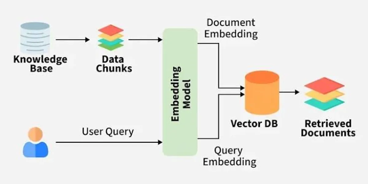
Almost every serious RAG system has the same backbone:

Ingestion
- Read docs from PDFs, wikis, repos, ticket systems.
- Normalize text, extract structure (headings, sections, metadata).
Chunking
- Split documents into smaller pieces that are:
  - precise enough to match a specific question,
  - but large enough to make sense on their own.
Embedding + Indexing
- Turn each chunk into an embedding vector.
- Store vectors and metadata in a vector database or index.
Retrieval
- Embed the user’s query.
- Search the index for the most relevant chunks.
- Optional: blend keyword search with semantic search, apply filters, rerank.
Generation
- Feed the retrieved chunks plus the question into the LLM.
- Instruct it to answer grounded in those chunks, with citations.
- Return the answer to the user.

Everything else (chunk overlap, hybrid search, reranking, etc.) is a refinement of one of these steps.

3. Chunking strategy: getting the “shape” right

Chunking strategy is how you cut long documents into smaller pieces before indexing.

You cannot paste a 400‑page handbook into a prompt. Even if you could afford it, the model answers worse when buried in noise. So you slice documents into chunks that are:

small enough to be precise,
large enough to be self‑contained.

3.1 Fixed-size vs structure-aware chunking

The naive approach:

Split every document into fixed 500‑character or 512‑token chunks.
It’s easy and often wrong:
- slices mid‑sentence,
- breaks tables and code blocks in half,
- separates headings from their contents.

A better approach respects structure:

Split on:
- headings and subheadings,
- paragraphs and sections,
- markdown blocks,
- function boundaries in code.
Keep each chunk aligned with a coherent unit of meaning.

A practical compromise many teams use today:

Recursive, token‑aware splitting:
- Start from top‑level sections (e.g., markdown headings).
- If a section is longer than your target size (say, 512 tokens), recursively split by smaller units (paragraphs, sentences).
This keeps boundaries clean without requiring full semantic parsing.

3.2 Chunk size heuristics

There is no universal perfect chunk size. It depends on your data and model context window. Modern benchmarks and RAG guides tend to use:

400–800 tokens for general documentation (SaaS docs, wikis).
200–400 tokens for highly structured reference docs (API specs, FAQs).
Larger chunks (800–1200 tokens) for narrative content (tutorials, long articles), where context matters more than pinpoint precision.

Treat these as starting points, not final truth. The right size is something you measure for your corpus.

4. Chunk overlap: boundary insurance, tuned by data

Chunk overlap repeats a small portion of text at the start of chunk i+1 that already appeared at the end of chunk i. Its only job is to protect you from boundary cuts that split a useful sentence across chunks.

If the answer to “How do I reset my password?” straddles the boundary between chunk 4 and chunk 5, neither chunk alone contains the full answer. A bit of overlap makes sure at least one chunk holds the complete thought.

4.1 When overlap helps

Overlap is most useful when:

You chunk by raw size (tokens, characters), not strict structure.
Your docs contain sentences or table rows whose meaning spans boundaries:
- technical manuals,
- legal contracts,
- dense analytical reports.

If you strictly chunk by headings or complete Q&A pairs, you may need very little overlap.

4.2 How much overlap (facts vs heuristics)

Recent 2025–2026 RAG evaluations mostly converge on:

10–20% of chunk size as a good starting range.
For a 512‑token chunk, that’s about 50–100 tokens of overlap.

Important: this is not a universal rule.

Too little overlap → boundary failures where key sentences are split.
Too much overlap → duplication:
- larger index,
- higher embed/storage cost,
- multiple near‑identical chunks in top‑k results.

The right value depends on your corpus. The way to find it is to:

fix chunk size,
sweep overlap (0%, 10%, 20%),
measure boundary recall and duplication on a small labeled question set.

5. Embeddings: meaning as numbers

Embeddings turn a piece of text into a vector of numbers that captures its meaning.

An embedding model reads a chunk and outputs an array of, say, 768 or 1536 floats.
Chunks with similar meaning produce vectors that are close to each other.
That’s why “How do I reset my password?” can match a doc titled “Credential recovery procedure” even though they share no words.

You use embeddings for:

every chunk at indexing time,
every query at search time.

Modern practice:

Use off‑the‑shelf embedding models (OpenAI, Cohere, open-source like E5, bge, GTE), not ones you train yourself.
The embedding model for your queries and documents must be the same.
Changing embedding models means re‑embedding and re‑indexing everything. Treat this choice like picking a database.

6. Vector databases: searching meaning at scale

A vector database is where you store those embedding vectors and find similar ones fast.

Comparing your query against every chunk one by one is fine for 1,000 chunks and unusable for 10 million. Vector databases use approximate nearest neighbor (ANN) indexes (like HNSW, IVF, etc.) to find the closest vectors in milliseconds without scanning all of them.

Common options:

Dedicated vector stores:
- Pinecone, Weaviate, Qdrant, Chroma.
Vector extensions to existing DBs:
- pgvector for Postgres,
- Milvus as a service or standalone.

A good rule of thumb:

If you’re already on Postgres and your corpus is under tens of millions of chunks, start with pgvector—one less system to operate.
For very large or latency‑critical workloads, dedicated vector stores may give better performance and features.

You don’t need to implement ANN yourself, but you should know:

It’s approximate by design—occasionally imperfect in exchange for big speed gains.
You control the tradeoff between recall and latency via index parameters.

7. Similarity search: how “closeness” is measured

Once everything is vectors, relevance becomes distance.

The most common metric is cosine similarity:

Think of vectors as arrows in high‑dimensional space.
Cosine similarity asks whether two arrows point in roughly the same direction.
Scores near 1.0 = very similar; near 0.0 = unrelated.

You rarely write this yourself (your library does), but you read the scores constantly when debugging.

Key practice:

Don’t treat similarity scores as absolute truth.
A “0.71” might be great in one corpus and useless in another.
Thresholds like “reject anything under 0.8” are dangerous unless you’ve plotted your own score histogram.

8. Top‑k: how many chunks you send to the model

Your retriever ranks every chunk by similarity, then you pick the top‑k.

k = 5 → top 5 chunks go into the prompt.
k = 10 → ten chunks, more context, more tokens.

k controls:

Quality: too low and the right passage never makes it in.
Cost: too high and you pay for tokens and latency.
Focus: too high and you bury the key chunk in mediocre ones.

Typical ranges:

k = 3–10 for direct question answering.
Larger k (20–50) when you plan to rerank and then narrow.

Common pattern:

Retrieve wide (k_raw ≈ 50).
Use a reranker to pick the best 5.
Pass those 5 to the LLM.

This lets you have both recall (wide retrieval) and precision (narrow prompt).

9. Hybrid search: combining keyword and semantic search

Semantic search (embeddings) is great for meaning and bad at exact strings. Keyword search is the opposite.

Ask about error code ERR_4021:

Pure semantic search might return something about “errors in general.”
Keyword search nails exact mentions of ERR_4021, but misses paraphrases.

Hybrid search runs both:

BM25 or similar keyword ranking.
Vector similarity search.

Then merges results so documents ranked highly by either method surface at the top.

You reach for hybrid search whenever your domain has:

product SKUs,
ticket numbers,
function names,
drug names,
legal citations,
internal acronyms.

In practice (2026), hybrid search plus reranking is often the biggest single quality jump for enterprise RAG.

10. Metadata filtering: narrowing to what’s allowed and relevant

Metadata filtering uses attributes stored alongside each chunk:

author,
department,
date,
customer ID,
document type,
access level.

Then it constrains retrieval:

“Only look in docs with customer_id = 123.”
“Only consider entries from last 6 months.”
“Only search internal ‘support’ space for this user.”

Without filtering:

Multi‑tenant products leak data across tenants.
Old docs override new ones.
Sensitive docs surface to unauthorized users.

Vector stores now widely support pre‑filtering:

Apply filters before ANN search, not after.
Avoid the situation where you retrieve 10 chunks, then filters remove 8, leaving 2 mediocre ones.

This is where your existing backend skills (access control, tenancy, schema design) are a big advantage.

11. Query rewriting: making messy user questions searchable

Real users type messy questions. They say:

“does it work with mine”

following three previous messages.

That string alone retrieves nothing useful. A query rewriter turns it into:

“Does the Pro plan support SAML single sign‑on?”

and suddenly retrieval works.

Two main flavors:

Contextual rewriting:
- Fold conversation history into a standalone query.
- Essential for multi‑turn chat: each new message is rewritten with previous turns applied.
Expansion:
- Generate a few paraphrases or synonym‑rich versions of the query.
- Search all of them and merge results.

This adds a small, fast model call before every search, so you:

use a lightweight model,
cache aggressively for repeated queries.

12. HyDE: hypothetical document embeddings (situational)

HyDE (Hypothetical Document Embeddings) is a specialized trick:

Ask the model to generate a fake answer to the question—like a mini doc that might contain the answer.
Embed that fake answer.
Use it as the search query.

Because answers look more like answers than questions do, this can improve retrieval when:

queries are short,
docs are dense and technical,
the corpora and question style differ strongly.

Trade‑offs:

You add a full generation before search → latency and cost.
It works well in some domains and not at all in others.

Treat HyDE as a situational tool, not a default. The right way to use it is:

implement it on top of your baseline,
measure whether it actually improves retrieval on your eval set,
keep it only if the gains are clear.

13. Reranking: a second, smarter pass

First‑stage retrieval is optimized for speed. It’s blunt. A reranker (cross‑encoder) takes the top 50 candidates and re‑scores them more carefully:

It reads query and document together.
It outputs a relevance score per pair.
You sort by those scores and keep the top few.

Typical pattern:

Retrieve 50 candidate chunks via embeddings.
Run a cross‑encoder reranker (e.g., Cohere Rerank, open models like bge-reranker).
Keep the top 5–10 for the LLM.

Because cross‑encoders are more accurate but slower, this “fast then slow” architecture gives you:

scalability (ANN for broad search),
precision (cross‑encoder for final ordering).

In real systems, reranking is often the highest quality‑per‑engineering‑hour upgrade in the entire pipeline.

14. Small‑to‑big retrieval (parent–child)

Small chunks match queries precisely but often lack context. Big chunks provide context but match less accurately. Small‑to‑big retrieval resolves this:

Index small chunks (sentences, small paragraphs).
Store a mapping from each small chunk to its parent section or “big” chunk.
At retrieval, search among small chunks.
When one hits, pass its parent section into the LLM.

This works extremely well for:

legal contracts,
technical manuals,
API references,
policy documents,

where a single sentence only makes sense within its surrounding heading and section.

Implementation is simple:

a parent_id field on each chunk,
one lookup after retrieval.

15. Contextual retrieval: giving chunks a “name tag”

Contextual retrieval prepends a short description of where a chunk came from before embedding it.

Example:

Without context:

revenue grew 12 percent
With context:

From the Q3 2024 earnings report, Northwind Systems, financial results section. Revenue grew 12 percent.

The second is easier to find and interpret:

Semantic search now sees “Q3 2024”, “Northwind Systems”, “financial results”.
Keyword search benefits from the added terms too.

Anthropic and others reported strong gains from this technique, and it’s now common in production systems for:

financial filings,
repeated report formats,
ticket histories,
meeting notes.

Usually:

you generate the context line once per chunk at ingestion time using a small model,
prepend it before embedding,
store the original text and the enriched text side by side.

16. Grounding and citations: making answers trustworthy

Grounding means forcing the model to answer only from retrieved text, and to admit when it doesn’t know.

Citations mean every claim points back to a specific source chunk.

Why this matters:

Models will happily invent confident but wrong answers when they don’t see relevant evidence.
In regulated or high‑stakes domains (legal, medical, finance), ungrounded answers are unacceptable.

A grounded RAG answer usually:

states the answer, and
lists one or more source passages (with doc names, IDs, or URLs).

Internally, you:

Give chunks stable identifiers (IDs or anchors).
Include those IDs in the prompt.
Ask the model to cite them.
Validate that cited IDs actually came from retrieval, not hallucination.

A system that reliably says:

“I couldn’t find this in your documentation.”

is more valuable than one that guesses slightly more often but sometimes fabricates.

17. Retrieval evaluation: turning intuition into evidence

Without evaluation, every change to your RAG system is a guess.

Two core questions:

Did retrieval find the right passages?
- Measured by recall@k:
  - For each question with a known ground‑truth chunk,
  - Did that chunk appear in the top‑k results at all?
Did the answer faithfully use those passages?
- Measured by faithfulness or supportedness:
  - Is every important claim traceable to retrieved evidence?

The most useful eval set is small and custom:

20–100 real questions from your domain.
For each:
- one or more “correct” chunks (doc ID + span),
- one or more acceptable answers.

Then, for every change (chunk size, overlap, hybrid search, reranker, filters), you:

re‑run retrieval on this test set,
compute recall@k and other metrics,
compare against the previous version.

Being able to say:

“Switching to recursive chunking with 15% overlap improved recall@5 by 12% on our docs.”

is the difference between tinkering and engineering.

18. A few important topics you shouldn’t skip

Beyond the concepts above, modern RAG systems benefit from a few additional practices:

18.1 Latency, caching, and cost

Cache:
- embeddings for repeated queries,
- retrieval results for hot questions,
- rewritten queries in multi‑turn chat.
Budget:
- how many tokens you can afford per request,
- how many model calls (rewriter, reranker, LLM) per pipeline.

RAG is usually I/O and model‑call heavy. Good caching and budgeting often matter as much as model choice.

18.2 Observability and logging

Treat your RAG pipeline like any distributed system:

log queries,
retrieved chunks,
similarity scores,
model inputs and outputs,
latency per stage.

This makes debugging “bad answer” reports far easier:

you can see whether retrieval, rewriting, or generation actually failed.

18.3 Safety and access control

RAG can surface sensitive information if you’re not careful. Combine:

metadata filtering (per‑tenant, per‑user),
content redaction where needed,
and output filters (e.g., for PII detection).

Modern RAG in enterprises lives inside a security and privacy boundary, not just a demo sandbox.

19. Putting it all together

You don’t need to memorize every term. The goal is to build one real system that touches most of them:

Pick a corpus you care about:
- your team’s docs,
- a framework you use,
- a folder of PDFs you keep rereading.
Ingest and chunk:
- use structure-aware, recursive chunking at ~512 tokens,
- start with 10–20% overlap and tune from there.
Embed and index:
- choose a solid embedding model,
- use pgvector or a simple vector store.
Build retrieval:
- semantic search,
- add hybrid search for IDs,
- add metadata filters for tenants and time.
Refine:
- query rewriting for multi‑turn chat,
- reranking for precision,
- small‑to‑big retrieval where context matters,
- contextual retrieval to make chunks identifiable.
Ground answers:
- enforce citations,
- handle “no answer found” gracefully.
Evaluate:
- write 20–50 evaluation questions,
- track recall@k and supportedness,
- use these metrics any time you change chunking, overlap, or search parameters.

That one project will give you more intuition than reading ten more blog posts—and it will give you something concrete to talk about when you explain your RAG experience to your users, your team, or future hiring managers.